Why Linear Regression is Called “Regression”: regression towards mediocrity

Introduction

Linear regression is a widely used statistical technique that aims to model the relationship between a dependent variable and one or more independent variables. It plays a crucial role in various fields, including economics, social sciences, healthcare, and engineering. But have you ever wondered why this powerful modeling technique is called “regression”?

In this blog post, we’ll explore the historical context behind its naming.

Context: Galton’s eugenicist quest

Francis Galton, a cousin of Charles Darwin, was deeply influenced by Darwin’s theory of evolution. Darwin’s theory centred around the survival of the fittest, suggesting that only the most adaptable species or groups would endure and reproduce. This theory was primarily concerned with animals and plants, but Galton was intrigued by its potential application to human beings, with the aim of advancing human biological development.

Galton held great admiration for Adolphe Quetelet, a Belgian statistician who popularized the concept of a normal distribution of human traits around an average value. Inspired by Quetelet’s work, Galton initially focused his research on geniuses, investigating the possible heredity of exceptional intellectual prowess by looking at famous families like the Bachs, Bernoullis, or Darwins. In his analysis, he emphasized biological inheritance over environmental influences such as education or upbringing, a view that contrasts with contemporary perspectives.

Since quantifying genius proved challenging, Galton decided to shift his focus to a more measurable trait: height.

Contrasting with Quetelet, Galton’s groundbreaking contribution was his perspective on the normal distribution of human characteristics and heredity. This gave rise to an apparent paradox (regression to the mean) that ultimately led to a new conceptual development: “regression” in its modern statistical sense.

Height between parents and son: a bivariate normal distribution

Data Description

Galton collected data on the heights of 930 children and of their respective parents, 205 in total.

Quote from [Galton, 1886]

My data consisted of the heights of 930 adult children and of their respective parentages, 205 in number. In every case I transmuted the female statures to their corresponding male equivalents and used them in their transmuted form, so that no objection grounded on the sexual difference of stature need be raised when I speak of averages. The factor I used was 1-08, which is equivalent to adding a little less than one-twelfth to each female height. It differs a very little from the factors employed by other anthropologists, who, moreover, differ a trifle between themselves; anyhow, it suits my data better than 107 or 109. The final result is not of a kind to be affected by these minute details, for it happened that, owing to a mistaken direction, the computer to whom I first entrusted the figures used a somewhat different factor, yet the result came out closely the same.

Empirical findings

Galton performed a cross-tabulation of the children’s height and the midparent’s height.

Do you notice any pattern in the cross-tabulation below? (Galton did!)

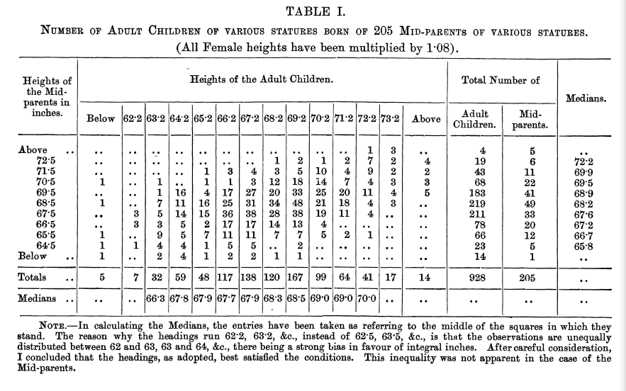
Cross-tabulation from [Galton, 1886]

On the cross-tabulation, he drew a line uniting boxes of the same value and noticed:

1. all the lines of same value have an ellipsis shape

2. the ellipsis are all centered on the point corresponding to the heights of the two generations

3. the points where each ellipse in succession was touched by a horizontal tangent, lay in a straight line inclined to the vertical in the ratio of 2/3

In his own words:

Quote from [Galton, 1886]

I found it hard at first to catch the full significance of the entries in the table, which had curious relations that were very interesting to investigate. They came out distinctly when I ” smoothed ” the entries by writing at each intersection of a horizontal column with a vertical one, the sum of the entries in the four adjacent squares, and using these to work upon. I then noticed (see Plate X) that lines drawn through entries of the same value formed a series of concentric and similar ellipses. Their common centre lay at the intersection of the vertical and horizontal lines, that corresponded to 68’ inches. Their axes were similarly inclined. The points where each ellipse in succession was touched by a horizontal tangent, lay in a straight line inclined to the vertical in the ratio of 2/3; those where they were touched by a vertical tangent lay in a straight line inclined to the horizontal in the ration of 1/3.

He summarized this finding in the following diagram:

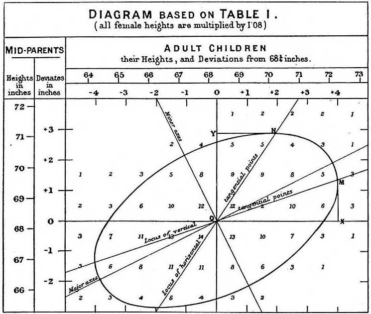
Diagram from [Galton, 1886]

Not knowing how to interpret them, he presented them to a mathematician, J. Hamilton Dickson. Dickson immediately recognized a two-dimensional normal law. We are going to explain in the next section the maths behind this phenomenon and how this is related to linear regression.

Mathematical formalization

Let’s consider the pair (X, Y) representing a child’s height and the mid-parent’s height, respectively.

What Galton empirically unveiled was that the pair (X, Y) adheres to a bivariate normal distribution.

Definition: bivariate normal distribution

Let (X, Y) follow a bivariate normal distribution. The probability density function is defined as :

\[f(z) = \frac{\exp^{\frac{-(z-m)^{t}C^{-1}(z-m)}{2}}}{2\pi\sqrt{det(C)}}\]

where \(C \in M_{2 \times 2}(\mathbb{R})\) is a positive definite symmetric matrix and \(m \in \mathbb{R}^{2}\) and \(z = (x y)\).

We can set:

\[\begin{split}C =\begin{bmatrix} \sigma_x^2 & \rho \sigma_x \sigma_y \\ \rho \sigma_x \sigma_y & \sigma_y^2 \\ \end{bmatrix}\end{split}\]

\[\begin{split}m =\begin{bmatrix} \mu_x \\ \mu_y \\ \end{bmatrix}\end{split}\]

One of Galton’s initial observations was that the lines of identical value exhibited an elliptical shape. In other words, we are looking for regions of equal density.

For a bivariate normal distribution, areas of uniform density (where k is held constant) can be expressed as:

\[f(x, y) = \frac{1}{2\pi \sigma_x \sigma_y \sqrt{1-\rho^2}} \exp{\frac{-k^{2}}{2}}\]

Equivalently, we are looking for regions where \(q(x,y) = (z-m)^{t}C^{-1}(z-m)= k^{2}\).

Since C is a positive definite symmetric matrix, according to the spectral theorem, there exists an orthogonal matrix P and a diagonal matrix D such that \(C = PDP^{t}\) where:

\[\begin{split}D =\begin{bmatrix} a^2 & 0 \\ 0 & b^2 \\ \end{bmatrix}\end{split}\]

If we define:

\[\begin{split}\begin{bmatrix} u \\ v\\ \end{bmatrix}=P(z-m)\end{split}\]

Using the orthogonal properties of P, this translates to a rotation in the \((x- \mu_x,y-\mu_y)\) plane, yielding the ellipsis \(q(x,y) = (z-m)^{t}C^{-1}(z-m) = k^{2} = \frac{u^{2}}{a^2} + \frac{v^{2}}{b^2}\).

This proves that if we have a bivariate normal distribution, the regions of equal density have the shape of an ellipsis.

Furthermore, the ellipses are centered around \((\mu_x, \mu_y)\) (which in our case represents the average heights of the children and parents respectively).

This is in line with the Galton’s first and second empirical evidence above!

Still, there remains the last empirical evidence: the points where each ellipse in succession was touched by a horizontal tangent, lay in a straight line inclined to the vertical in the ratio of 2/3 (which represents the coefficient of the linear regression when regressing children’s height based on parents’ height).

To elucidate this, let’s differentiate: \(\frac{\delta q(x,y)}{\delta y}=0\).

Which leads to (drumroll), a simple linear regression equation: \(y = \mu_y + \rho \frac{\sigma_y}{\sigma_x} (x - \mu_x)\).

We’ve demonstrated that the observed empirical evidence arises from the bivariate normal distribution between the heights of children and their parents. Furthermore, we begin to discern a connection with the contemporary understanding of linear regression.

In the following section, we will explore how this research, via the notion of regression to mediocrity, has paved the way for our current usage of the term “regression.”

Regression to the mean/mediocrity

Galton observed that tall parents tended to have children who, on average, were shorter than their parents.

Conversely, short parents often had children who were taller than they were.

He found that the difference between a parent’s height and the population’s average height was reduced by about 2/3 in their offspring. For example, if the average population height was 66 inches and a parent was 72 inches tall (6 inches above average), their child would be expected to be, on average, 2/3 x 6 inches = 4 inches above the population average, or 70 inches tall.

Galton termed this phenomenon “regression to mediocrity,” which has since been renamed as “regression to the mean”.

The term “mediocrity” here refers to the average or the mean, as Galton was interested in the extreme right tail of the distribution (tallest people). So, the phrase “regression towards mediocrity” described the observed phenomenon that offspring tended to be closer to the average height of the population than their parents were.

It’s crucial to note that “regression to the mean” doesn’t mean that over time everything becomes average. It’s a statistical effect that refers to the fact that if a variable is extreme the first time you measure it, it will be closer to the average the next time you measure it.

Mathematically, we have seen that the pair (child height, average parents height) follow a bivariate normal distribution.

Given that:

\[f^{Y}_{\{X=x\}}(y) =: f(y|x) = \frac{f(x,y)}{f_{X}(x)}\]

We obtain for a normal distribution the linear relationship:

\[E(Y=y|X=x) =: \mu_{y|x} = y = \mu_y + \rho \frac{\sigma_y}{\sigma_x} (x - \mu_x)\]

Here Y represent a child’s height, and X represent the average parents’ height.

Since height is stationary (its distribution does not change much over time), the average height population is roughly the same between generations \(\mu_y= \mu_x =\mu\).

So we obtain \((y-\mu) = \rho \frac{\sigma_y}{\sigma_x}(x-\mu) = \frac{2}{3}(x-\mu)\).

Therefore \(E(Y=y|X=x) = \frac{2}{3}x + (1-\frac{2}{3})\mu\).

If we want to go into more details \(\sigma_y= \sqrt{2}\sigma_x\), since:

1. \(X = \frac{X_1 + X_2}{2}\)

2. \(Var(X_1) = Var(X_2) = Var(Y)\)

3. \(X_1 \perp \!\!\! \perp X_2\)

Link with modern regression analysis

In a regression problem with some explanatory variables X, and a response variable Y, we usually decompose Y as:

\[ \begin{align}\begin{aligned}Y_i = E(Y_i|X_i) + \epsilon_i\\\text{where} E(\epsilon_i|X_i)=0\end{aligned}\end{align} \]

With this decomposition we then try to model \(E(Y_i|X_i)\).

The justification of using \(E(Y_i|X_i)\) is that it is the best predictor of \(Y_i\) given \(X_i\), in the sense that it solves a Minimum Mean Squared Error (MMSE) prediction problem:

Let \(m(X_i)\) be any function of \(X_i\):

\[E[Y_i | X_i] = \arg\min_{m(X_i)} E \left[ (Y_i - m(X_i))^2 \right]\]

When we use a linear regression, we are assuming that \(E(Y_i|X_i)\) is linear.

Under some circumstances like the one Galton has encountered (which is the multivariate normal distribution), \(E(Y_i|X_i)\) is linear.

In general, we can just interpret linear regression as the best linear estimate in the sense that it solves a Minimum Mean Squared Error (MMSE) prediction.

In other words, we restrict \(m(X_i)\) above to be any linear function.

How can we apply the concept of regression to the mean in life?

This principle can be applied in a number of everyday life situations:

1. Sports: After an unusually good season, a player is often expected to perform at the same high level or even better in the next season. However, often the player’s performance may decline or move towards their career average. This is not necessarily a reflection of a decline in the player’s abilities, but rather a statistical phenomenon of regression towards the mean.

2. Business: If a company has an extraordinarily good financial year, expectations might be that the following year would be just as good or even better. However, it’s more likely the following year’s performance will be closer to the company’s long-term average performance.

3. Health: In medical treatments, patients with severe symptoms tend to show more improvement than those with mild symptoms. This isn’t necessarily because the treatment is more effective on severe cases, but because severe cases have more room for improvement, which results in regression towards the mean.

4. Education: A student may score very high on a test. However, on the next test, their score may decrease to a value closer to their average score. This does not necessarily reflect a decrease in understanding or effort, but is often a natural statistical occurrence of regression towards the mean.

5. Investing: An investment might do exceptionally well one year, prompting you to expect it to continue doing well. But often, it will return closer to the average market return the next year.

In each of these cases, understanding regression to the mean helps temper expectations and reduces the likelihood of making decisions based on anomalies rather than long-term trends. It also encourages individuals to examine a broader set of data rather than focusing on one or two extreme data points.

Conclusion

The name “regression” in linear regression traces its roots back to the pioneering work of Francis Galton, who was deeply influenced by Darwin’s theory of evolution and was keen to explore its implications on human development.

Through his empirical study of height among parents and their offspring, Galton discerned a phenomenon he termed “regression towards mediocrity” – a tendency for offspring to be closer to the average height of the general population than their parents.

During his study, Galton discovered a bivariate normal distribution linking children’s heights to their parents’. This finding established a linear relationship between the expected child’s height and the height of their parents.

Modern linear regression analysis owes its terminology and foundational principles to Galton’s early exploration. While the implications of “regression towards mediocrity” extend beyond height, its mathematical formulation serves as the backbone for contemporary statistical modeling techniques.

In essence, Galton’s quest has left an enduring legacy in the world of statistics, shaping our understanding of relationships between variables.

References

AP09

Joshua D Angrist and Jörn-Steffen Pischke. Mostly harmless econometrics: An empiricist's companion. Princeton university press, 2009.

App13

Walter Appel. Probabilités pour les non-probabilistes. H&K éditions, 2013.

Desrosieres98

Alain Desrosières. The politics of large numbers: A history of statistical reasoning. Harvard University Press, 1998.

Gal86(1,2,3,4)

Francis Galton. Regression towards mediocrity in hereditary stature. The Journal of the Anthropological Institute of Great Britain and Ireland, 15:246–263, 1886.

How to cite this post?

@article{filali2023regression,
  title   = "Why Linear Regression is Called 'Regression': regression towards mediocrity",
  author  = "FILALI BABA, Hamza",
  journal = "hamzaonai.com",
  year    = "2023",
  month   = "July",
  url     = "https://hamzaonai.com/blog/why_linear_regression_called_regression.html"
}

Previous: How to reduce the amount of labelled data required for your Deep Learning model with a human in the loop?   Next: Detecting Trend Changes in Time-Series Data: A Frequentist and Parametric Approach

Comments

comments powered by Disqus