Detecting Trend Changes in Time-Series Data: A Frequentist and Parametric Approach

Introduction

Detecting trend changes in time-series can offer valuable insights for various applications. There are multiple ways to approach this problem, and each method comes with its own set of assumptions and intricacies.

This post aims to explore one such method—employing frequentist and parametric techniques to identify change-points in time-series data. While there are numerous non-parametric and Bayesian methods available, the focus here is on methods that utilize linear regression as a foundation.

We’ll walk you through two different model specifications—one allowing for changes in both the intercept and the slope, and another that focuses solely on the slope. By the end of this article, you will have learned how to construct hypotheses tests to assess the presence of structural changes and how to carry out these tests using Ordinary Least Squares (OLS) estimators.

Prerequisite knowledge in linear regression will be helpful to get the most out of this post.

Now, let’s delve into the specifics and learn how to identify those crucial turning points in your time-series data.

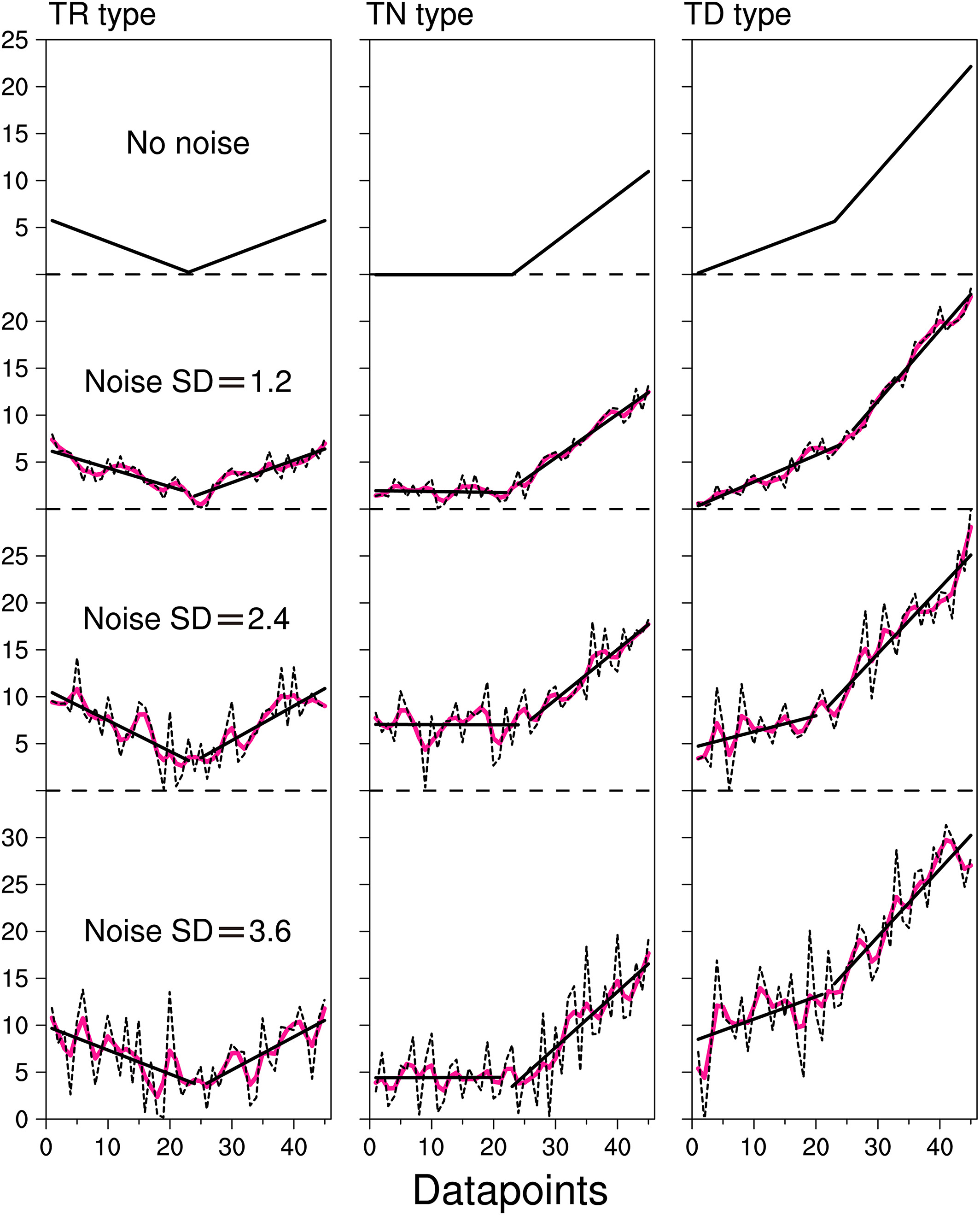
Illustration of different type of trend changes (source [Zuo et al., 2020])

How to detect trend changes in time series

Consider a time-series $\{y_t{\}}_1^{n+m}$, where the objective is to test for a trend change at time $n$. We are going to show two piecewise linear model specifications:

Step 1: define your linear model: unknown parameters + design matrix

Model 1 (Structural change in both intercept and slope)

$$y_t=({\mu }_0+{\beta }_{0}t){\mathbb{1}}_{t\le n}+({\mu }_1+{\beta }_{1}t){\mathbb{1}}_{t>n}+{ϵ}_t$$

This specification allows for a simultaneous change in the intercept and slope.

Unknown Parameters

$$\begin{array}{r}\beta =\left[\begin{array}{c}{\mu }_0\\ {\beta }_0\\ {\mu }_1\\ {\beta }_1\end{array}\right]\end{array}$$

Design Matrix

$$\begin{array}{r}X=\left[\begin{array}{cccc}1& 1& 0& 0\\ 1& 2& 0& 0\\ ⋮& ⋮& ⋮& ⋮\\ 1& n& 0& 0\\ 0& 0& 1& 1\\ 0& 0& 1& 2\\ ⋮& ⋮& ⋮& ⋮\\ 0& 0& 1& m\end{array}\right]\end{array}$$

Model 2 (Structural change in slope)

This specification allows for a one-time change in the slope of the trend without affecting the level. In mathematical terms, the model can be represented as:

$$y_t=\mu +{\beta }_{0}t{\mathbb{1}}_{t\le n}+{\beta }_{1}t{\mathbb{1}}_{t>n}+{ϵ}_t$$

Step 2: Define Your Testing Hypothesis

There are several tests that can be formulated to assess whether a structural change has occurred in the time series. Depending on the specific aspect you want to test, the null hypothesis (H0) could take various forms. In the case of Model 1, for example, you could consider:

1. $H_0:{\beta }_0={\beta }_1$ which tests for equality between the slopes before and after the change point.

2. $H_0:{\beta }_0={\beta }_1\text{ and }{\mu }_0={\mu }_1$. This is a joint hypothesis which tests for equality in both the slope and the intercept at the time $n$.

If either of these null hypotheses is rejected, it would imply that a structural change has occurred at the change point $n$.

In a more generalized form, these hypotheses can be expressed as:

$$H_0:R\beta =r$$

Here, $R\in M_{jq}(\mathbb{R})$ is a matrix that linearly transforms the parameter vector $\beta$, and $r$ is a constant vector. The exact forms of $R$ and $r$ will depend on the hypothesis you’re testing. For example:

• For the first test $H_0:{\beta }_0={\beta }_1$, $R$ could be a row vector $[0,-1,0,1]$ and $r$ would be $[0]$.

• For the second joint hypothesis $H_0:{\beta }_0={\beta }_1\text{ and }{\mu }_0={\mu }_1$, $R$ could be a matrix

$$\begin{array}{r}\left(\begin{array}{cccc}1& 0& -1& 0\\ 0& 1& 0& -1\end{array}\right)\text{and }r\text{ would be }[0,0].\end{array}$$

This flexible framework allows for various types of hypotheses to be tested, depending on your specific research questions and the data at hand.

Step 3: Construct your test

For a given hypothesis expressed above, we are going to see how to test the above generalized from hypothesis using OLS estimators.

To test the null hypothesis $H_0:R\beta =r$, where $r$ is a ( j times 1 ) non-random vector, the Wald statistic is defined as follows:

$$W_N=(R{\hat{\beta }}_N-r{)}^T{\left[R\left(\frac{{\hat{V}}_N}{N}\right)R^T\right]}^{-1}(R{\hat{\beta }}_N-r)$$

Here, ${\hat{V}}_N$ is the estimated covariance matrix, $N$ is the sample size, ${\hat{\beta }}_N$ is the estimated parameter vector, and $R$ is the matrix indicating linear restrictions on $\beta$.

We are going to see that under the null hypothesis $H_0$, the Wald statistic $W_N$ is asymptotically distributed as a chi-square distribution with $j$ degrees of freedom, i.e., $W_N\stackrel{a}{\to }{\chi }_j^2$.

In finite sample, under $H_0$, we make the following approximation: $W_N\approx {\chi }_j^2$.

Wald test

OLS reminder

As a reminder OLS estimation consists in: $\hat{\beta }=\arg \underset{\beta }{min}\Vert Y-X\beta {\Vert }^2$.

We obtain the estimator:

$$\begin{array}{rl}\hat{\beta }& =(X^{t}X{)}^{-1}(X^{t}Y)\\ & =\beta +(\frac{X^{t}X}{N}{)}^{-1}(\frac{X^t\widehat{ϵ}}{N})\\ & =(\frac{\sum _{i=1}^N{x}_i^t{x}_i}{N}{)}^{-1}(\frac{\sum _{i=1}^N{x}_i^t{y}_i}{N})\\ & =\beta +(\frac{\sum _{i=1}^N{x}_i^t{x}_i}{N}{)}^{-1}(\frac{\sum _{i=1}^N{x}_i^t{\widehat{ϵ}}_i}{N})\end{array}$$

From the expression above, we obtain the following decomposition:

$$\begin{array}{r}\sqrt{N}(\hat{\beta }-\beta )=\underset{\begin{array}{c}\stackrel{P}{\to }E(X^{t}X{)}^{-1}\\ \text{Assuming we can use the law of large number}\end{array}}{\underbrace{(\frac{\sum _{i=1}^N{x}_i^t{x}_i}{N}{)}^{-1}}}\underset{\begin{array}{c}\stackrel{L}{\to }\mathcal{N}\mathcal{(}\mathcal{0}\mathcal{,}\mathcal{S}\mathcal{)}\text{ where S is a semidefinite positive matrix}\\ \text{ Assuming we can apply a central limit theorem on }{x}_i^t\widehat{{ϵ}_i}\text{ and }E(x^t\widehat{ϵ})=0\end{array}}{\underbrace{\sqrt{N}(\frac{\sum _{i=1}^N{x}_i^t\widehat{{ϵ}_i}}{N})}}\end{array}$$

By applying Slutsky’s theorem, we get: $\sqrt{N}(\hat{\beta }-\beta )\stackrel{L}{\to }\mathcal{N}(0,E(X^{t}X{)}^{-1}SE(X^{t}X{)}^{-1})$.

Let V denote $E(X^{t}X{)}^{-1}SE(X^{t}X{)}^{-1}$, we get $R\sqrt{N}(\hat{\beta }-\beta )\stackrel{a}{\sim }\mathcal{N}(0,RV{R}^t)$.

It follows that $R\sqrt{N}(\hat{\beta }-\beta )(RV{R}^t{)}^{-1}(R\sqrt{N}(\hat{\beta }-\beta ))\stackrel{a}{\sim }{\chi }_j^2$.

If we can find an estimator of V, i.e. $\widehat{V_n}\stackrel{P}{\to }V$, then $R\sqrt{N}(\hat{\beta }-\beta )(R\widehat{V_n}{R}^t{)}^{-1}(R\sqrt{N}(\hat{\beta }-\beta ))\stackrel{a}{\sim }{\chi }_j^2$.

For a detailed explanation, please refer to chapter 3 and 4 of Wooldridge’s “Econometric Analysis of Cross Section and Panel Data” [Wooldridge, 2010] or chapter 5 of [Greene, 2003].

Let’s recap:

1. Assumption 1: $E(x^tϵ)=0$ (often referred as OLS 1, e.g. in [Wooldridge, 2010])

2. Some form of Law of Large Numbers and Central Limit Theorem can be applied. Please refer to [White, 2014] to look at the appropriate one to use.

3. We need to find an estimator ${\hat{V}}_N$ of $V$. As a reminder, $V=E(X^{t}X{)}^{-1}E(X^tϵ{ϵ}^{t}X)E(X^{t}X{)}^{-1}$. The main work lies in making the right assumption of the structure of $ϵ$ to estimate $S=E(X^tϵ{ϵ}^{t}X)$.

4. Under $H_0$, $W_N\approx {\chi }_j^2$

What could be a good covariance matrix estimator?

Let’s start simple: Homoscedasticity assumption

In linear regression we often make the Homoscedasticity assumption $E(ϵ{ϵ}^t|X)={\sigma }^{2}I$ .

It follows that $V=E(X^{t}X{)}^{-1}E(E(X^tϵ{ϵ}^{t}X|X))E(X^{t}X{)}^{-1}={\sigma }^{2}E(X^{t}X{)}^{-1}E(X^{t}X)E(X^{t}X{)}^{-1}={\sigma }^{2}E(X^{t}X{)}^{-1}$.

A natural unbiased estimator of ${\sigma }^2$ is ${\hat{\sigma }}^2=\frac{{\widehat{ϵ}}^t\widehat{ϵ}}{n-q}$.

$\text{On estimating }{\sigma }^2$

Let’s show that $E({\widehat{ϵ}}^t\widehat{ϵ})=(n-q){\sigma }^2$

Since, $\widehat{ϵ}=Y-X\hat{\beta }=(I-X(X^{t}X{)}^{-1}{X}^t)Y=(I-X(X^{t}X{)}^{-1}{X}^t)ϵ$.

By denoting $M=I-X(X^{t}X{)}^{-1}{X}^t$, we get: ${\widehat{ϵ}}^t\widehat{ϵ}={ϵ}^t{M}^{t}Mϵ={ϵ}^{t}Mϵ$.

Because ${ϵ}^{t}Mϵ$ is a scalar, it follows that:

$tr({ϵ}^{t}Mϵ)=tr(Mϵ{ϵ}^t)={\sigma }^{2}tr(M)$

And we get that $tr(M)=tr(I_n-X(X^{t}X{)}^{-1}X)=n-tr(X(X^{t}X{)}^{-1}{X}^t)=n-tr(I_q)=n-q$

Hence the unbiased estimator ${\hat{\sigma }}^2=\frac{{\widehat{ϵ}}^t\widehat{ϵ}}{n-q}$.

If we assume further that the error terms are normally distributed, leveraging $\widehat{ϵ}{\widehat{ϵ}}^t=ϵM{ϵ}^t$ and using the property below, we get that ${\hat{\sigma }}^2\sim {\chi }_{n-q}^2$

Chi square property

$$\text{If }u\sim \mathcal{N}(0,I_n)\text{ and }A\text{ is an }n\times n\text{ symmetric, idempotent matrix with }\text{rank}(A)=q,\text{ then }{u}^{T}Au\sim {\chi }_q^2$$

We obtain that $F=\frac{W}{j}\frac{{\sigma }^2}{{\hat{\sigma }}^2}\sim F_{j,n-q}$ under $H_0$.

In finite sample, $F_N=\frac{(R{\hat{\beta }}_N-r{)}^T{[R(X^{t}X{)}^{-1})R^T]}^{-1}(R{\hat{\beta }}_N-r)}{j{\hat{\sigma }}^2}\approx F_{j,N-q}$

F-distribution definition

$\text{Let }{X}_1\sim {\chi }_{q_1}^2,X_2\sim {\chi }_{q_2}^2$. $\text{Assuming }{X}_1\perp X_2$. $F=\frac{\frac{X_1}{q_1}}{\frac{X_2}{q_2}}$ has an F distribution with $(q_1,q_2)$ degrees of freedom. We denote this as $F\sim F_{q_1,q_2}$

Note 1: Relation with t-test

You might be more familiar with t-tests. If j=1, $\sqrt{F}=T\sim t_{n-q}$.

Note 2: on the normality assumption

One point to note is that the necessity for the normality assumption decreases as the sample size increases. If we have a very large sample size, the Wald statistic can be used directly without turning it into an approximate F-distribution.

Newey-West Estimator

But in time-series analysis, it’s generally unrealistic to assume that error terms are uncorrelated across time. Wooldridge illustrates in Chapter 12 of his book how traditional estimators can be misleading under these circumstances. Specifically, he provides an example where the error term follows an AR(1) process with a positive coefficient. In such a scenario, conventional estimators that assume uncorrelated errors would underestimate the true standard errors, leading to incorrect inferences [Wooldridge, 2015].

We would like an estimator that is:

1. robust to heteroscedasticity and autocorrelation of error terms

2. semidefinite positive (otherwise some linear combination of the elements of $(x_i^t{ϵ}_i{)}_i$ is asserted to have a negative variance, which is problematic for an estimator of a variance-covariance matrix)

To meet these requirements, Newey and west suggested the following estimator ([Newey and West, 1987]):

$${\hat{S}}_N=\frac{\sum _{t=1}^N{ϵ}_t^2{x}_t^t{x}_t+\sum _{l=1}^L(1-\frac{l}{L+1})(\sum _{t=l}^N{x}_t^t{ϵ}_t{ϵ}_{t-l}{x}_{t-l}\sum _{t=l}^N{x}_{t-l}^t{ϵ}_{t-l}{ϵ}_t{x}_t)}{N}$$

We therefore get:

$$\frac{{\hat{V}}_N}{N}=(\sum _{t=1}^N{x}_t^t{x}_t{)}^{-1}(\sum _{t=1}^N{ϵ}_t^2{x}_t^t{x}_t+\sum _{l=1}^L(1-\frac{l}{L+1})(\sum _{t=l}^N{x}_t^t{ϵ}_t{ϵ}_{t-l}{x}_{t-l}\sum _{t=l}^N{x}_{t-l}^t{ϵ}_{t-l}{ϵ}_t{x}_t))(\sum _{t=1}^N{x}_t^t{x}_t{)}^{-1}$$

Application: Example with model 1

Running Slope Difference (RSD) Test

In [Zuo et al., 2019], the following test is suggested:

$$\begin{array}{r}\begin{array}{c}t=\frac{{\hat{\beta }}_1-{\hat{\beta }}_0}{\sqrt{\frac{C}{N-4}(\sum _{i=1}^n(y_i-{\hat{y}}_i{)}^2+\sum _{i=1}^{M-n}(y_{i+n}-{\hat{y}}_{i+n}{)}^2)}}\\ \text{where }C=\frac{1}{\sum _{i=1}^n(i-\frac{n+1}{2}{)}^2}+\frac{1}{\sum _{i=1}^m(i-\frac{m+1}{2}{)}^2}\end{array}\end{array}$$

where $t$ follows a T distribution with N-4 degrees of freedom under $H_0$

While the paper does not use matrix formualtion, we are going to see how we can obtain this result.

Problem reformulation

The paper does not use a matrix form like we do, but the formalization of their problem can be reformulated using Model 1 (Structural change in both intercept and slope) :

$$\begin{array}{r}\begin{array}{c}{y}_t=({\mu }_0+{\beta }_{0}t){\mathbb{1}}_{t\le n}+({\mu }_1+{\beta }_{1}t){\mathbb{1}}_{t>n}+{ϵ}_t\\ \begin{array}{c}\end{array}\\ \text{Our testing Hypothesis is: }{H}_0:{\beta }_0={\beta }_1\text{ (i.e. no trend change)}\\ \begin{array}{c}\\ \text{Which we express as: }R\beta =0,\text{ where }\beta =\left(\begin{array}{c}{\mu }_0\\ {\beta }_0\\ {\mu }_1\\ {\beta }_1\end{array}\right),R=\left(\begin{array}{cccc}0& 1& 0& -1\end{array}\right)\end{array}\end{array}\end{array}$$

Let’s see if we find obtain the same results.

$$\begin{array}{rl}{F}_N& =\frac{(R{\hat{\beta }}_N-r{)}^T{[R(X^{t}X{)}^{-1}{R}^T]}^{-1}(R{\hat{\beta }}_N-r)}{j{\hat{\sigma }}^2}\\ & =\frac{({\hat{\beta }}_1-{\hat{\beta }}_0{)}^2}{[R(X^{t}X{)}^{-1}{R}^T]{\hat{\sigma }}^2}\text{ (Since }j=1,[R(X^{t}X{)}^{-1}{R}^T]\text{ is a scalar)}\end{array}$$

All that is left to compute is: $(X^{t}X{)}^{-1}$ and ${\hat{\sigma }}^2=\frac{\widehat{ϵ}{\widehat{ϵ}}^t}{N-4}$

$(X^{t}X{)}^{-1}=C$

$$\begin{array}{r}\begin{array}{c}\begin{array}{c}{X}^{t}X=\left[\begin{array}{cc}A(n)& 0_{2,2}\\ 0_{2,2}& A(m)\end{array}\right]\end{array}\\ \begin{array}{rlr}\text{where}{A}_n=& \left[\begin{array}{cc}\sum _{i=1}^{n}1& \sum _{i=1}^{n}i\\ \sum _{i=1}^{n}i& \sum _{i=1}^n{i}^2\end{array}\right]=& \left[\begin{array}{cc}n& \frac{n(n+1)}{2}\\ \frac{n(n+1)}{2}& \frac{n(n+1)(2n+1)}{6}\end{array}\right]\end{array}\end{array}\end{array}$$

Since:

1. $\sum _{i=1}^{n}i=\frac{n(n+1)}{2}$

2. $\sum _{i=1}^n{i}^2=\frac{n(n+1)(2n+1)}{6}$

3. $n(\sum _{i=1}^n{i}^2)-(\sum _{i=1}^{n}i{)}^2=\frac{n^2(n+1)(n-1)}{12}=n\sum _{i=1}^n(i-\frac{n+1}{2}{)}^2$

We get:

$$\begin{array}{r}\begin{array}{c}\begin{array}{rlrl}A(n{)}^{-1}=& \left[\begin{array}{cc}\sum _{i=1}^n{i}^2& -\sum _{i=1}^{n}i\\ -\sum _{i=1}^{n}i& \sum _{i=1}^{n}1\end{array}\right]\times \frac{1}{n\sum _{i=1}^n(i-\frac{n+1}{2}{)}^2}=& \left[\begin{array}{cc}\frac{4n+2}{n(n-1)}& -\frac{6}{n(n-1)}\\ -\frac{6}{n(n-1)}& \frac{12}{n(n+1)(n-1)}\end{array}\right]=& \left[\begin{array}{cc}\frac{4n+2}{n(n-1)}& -\frac{6}{n(n-1)}\\ -\frac{6}{n(n-1)}& \frac{1}{\sum _{i=1}^n(i-\frac{n+1}{2}{)}^2}\end{array}\right]\end{array}\\ \text{Hence, }[R(X^{t}X{)}^{-1}{R}^T]=\frac{1}{\sum _{i=1}^n(i-\frac{n+1}{2}{)}^2}+\frac{1}{\sum _{i=1}^m(i-\frac{m+1}{2}{)}^2}=C\end{array}\end{array}$$

${\hat{\sigma }}^2=\frac{{\widehat{ϵ}}^t\widehat{ϵ}}{N-4}$

$${\widehat{ϵ}}^t\widehat{ϵ}=(Y-\hat{Y}{)}^t(Y-\hat{Y})$$

Hence, $F_N=\frac{({\hat{\beta }}_1-{\hat{\beta }}_0{)}^2}{\frac{C}{N-4}(\sum _{i=1}^n{y}_i-{\hat{y}}_i{)}^2+\sum _{i=1}^{M-n}(y_{i+n}-{\hat{y}}_{i+n}{)}^2)}$

$t=\sqrt{F_N}\approx t_{N-4}$ under $H_0$ :).

Bonus: simple code to implement the the RSD-test

Code snippet

from typing import Union, List, Dict, Optional
import numpy as np
from scipy import stats
from statsmodels.tsa.stattols import acf


def slope_difference_test(
    univariate_timeseries: Union[List[float], np.ndarray],
    separation_point: int,
    robust: Optional[bool] = True,
) -> Dict:
    """
    Statistical test for slop difference described in the following paper:
    Zuo, Bin, et al. "A new statistical method for detecting trend turning."
    Theoretical and Applied Climatology 138.1 (2019): 201-213.
    The null hypothesis is : no-slope difference between the two segments of the time series
    Parameters
    univariate_timeseries : 1d numpy array of shape (length_timeseries,)
    separation_point: Point on which we test if there is a trend shift
    Returns
    p_value : p value
    """
    min_float = 1e-10
    # Creating the left and the right window for slope detection
    l_window = univariate_timeseries[:separation_point]
    r_window = univariate_timeseries[separation_point:]
    l_window_length = len(l_window)
    r_window_length = len(r_window)
    ts_length = l_window_length + r_window_length
    eff_df = 4
    if robust:
        # Finding the effective degrees of freedom
        auto_corr = acf(univariate_timeseries, nlags=ts_length)
        auto_corr[np.isnan(auto_corr)] = 1
        for i in range(1, ts_length):
            eff_df = eff_df + (
                ((ts_length - i) / float(ts_length)) * auto_corr[i]
            )
            eff_df = max(
                1,
                int(
                    np.rint(
                        1
                        / (
                            (1 / float(ts_length))
                            + ((2 / float(ts_length)) * eff_df)
                        )
                    )
                ),
            )
    # Creating the left and right indices for running the regression
    l_x, r_x = np.arange(l_window_length), np.arange(
        r_window_length
    )
    # Linear regression on the left and the right window
    (
        l_slope,
        l_intercept,
        l_r_value,
        l_p_value,
        l_std_err,
    ) = stats.linregress(l_x, l_window)
    (
        r_slope,
        r_intercept,
        r_r_value,
        r_p_value,
        r_std_err,
    ) = stats.linregress(r_x, r_window)
    # t-test for slope shift
    l_window_hat = (l_slope * l_x) + l_intercept
    r_window_hat = (r_slope * r_x) + r_intercept
    l_sse = np.sum((l_window - l_window_hat) ** 2)
    r_sse = np.sum((r_window - r_window_hat) ** 2)
    l_const = (
        l_window_length
        * (l_window_length + 1)
        * (l_window_length - 1)
        / 12
    )
    r_const = (
        r_window_length
        * (r_window_length + 1)
        * (r_window_length - 1)
        / 12
    )
    C = (l_const * r_const) / (l_const + r_const)
    total_sse = l_sse + r_sse
    std_err = max(
        np.sqrt(
            total_sse
            / (C * (l_window_length + r_window_length - 4))
        ),
        min_float,
    )
    t_stat = abs(l_slope - r_slope) / std_err
    p_value = (1 - stats.t.cdf(t_stat, df=ts_length - eff_df)) * 2
    if np.isnan(p_value):
        p_value = 1
    return {
        "p_value": p_value,
        "t_stat": t_stat,
        "l_slope": l_slope,
        "l_intercept": l_intercept,
        "r_slope": r_slope,
        "r_intercept": r_intercept,
        "separation_point": int(separation_point),
        "l_r_value": l_r_value,
        "r_r_value": r_r_value,
    }

Conclusion

The test framework we’ve established is valid under the assumption that our error term is stationary.

For extensions beyond the stationary error term assumption, consider consulting the work by Pierre Perron, which proposes a test that accommodates an I(1) error term ([Perron and Yabu, 2009]).

References

Gre03

William H Greene. Econometric analysis. Pearson Education India, 2003.

Ham20

James D Hamilton. Time series analysis. Princeton university press, 2020.

NW87

Whitney K Newey and Kenneth D West. Hypothesis testing with efficient method of moments estimation. International Economic Review, pages 777–787, 1987.

PY09

Pierre Perron and Tomoyoshi Yabu. Testing for shifts in trend with an integrated or stationary noise component. Journal of Business & Economic Statistics, 27(3):369–396, 2009.

Whi14

Halbert White. Asymptotic theory for econometricians. Academic press, 2014.

Woo10(1,2)

Jeffrey M Wooldridge. Econometric analysis of cross section and panel data. MIT press, 2010.

Woo15

Jeffrey M Wooldridge. Introductory econometrics: A modern approach. Cengage learning, 2015.

ZHZ+20

Bin Zuo, Zhaolu Hou, Fei Zheng, Lifang Sheng, Yang Gao, and Jianping Li. Robustness assessment of the rsd t-test for detecting trend turning in a time series. Earth and Space Science, 7(5):e2019EA001042, 2020.

ZLSZ19

Bin Zuo, Jianping Li, Cheng Sun, and Xin Zhou. A new statistical method for detecting trend turning. Theoretical and Applied Climatology, 138(1):201–213, 2019.

Previous: Why Linear Regression is Called “Regression”: regression towards mediocrity   Next: Mistral 7B: Decoding the Complexities of a Large Autoregressive Language Model

Comments