Mistral 7B: Decoding the Complexities of a Large Autoregressive Language Model#
Introduction#
The goal of this post is to offer a clear understanding of how large language models like Mistral work ([Jiang et al., 2023]).
This post will cover:
The architecture of Mistral, highlighting its decoder-only setup.
Key functionalities like the sliding window attention mechanism and key-value cache.
An exploration of crucial implementation aspects, including the use and significance of the attention mask.
Our insights will be derived from examining Mistral’s implementation from 🤗 Hugging Face library.
We will be using transformers==4.35.0
Code snippet
from transformers import AutoModelForCausalLM, AutoTokenizer
model = AutoModelForCausalLM.from_pretrained("mistralai/Mistral-7B-v0.1")
tokenizer = AutoTokenizer.from_pretrained("mistralai/Mistral-7B-v0.1")

print(model)
MistralForCausalLM(
  (model): MistralModel(
    (embed_tokens): Embedding(32000, 4096)
    (layers): ModuleList(
      (0-31): 32 x MistralDecoderLayer(
    (self_attn): MistralFlashAttention2(
      (q_proj): Linear(in_features=4096, out_features=4096, bias=False)
      (k_proj): Linear(in_features=4096, out_features=1024, bias=False)
      (v_proj): Linear(in_features=4096, out_features=1024, bias=False)
      (o_proj): Linear(in_features=4096, out_features=4096, bias=False)
      (rotary_emb): MistralRotaryEmbedding()
    )
    (mlp): MistralMLP(
      (gate_proj): Linear(in_features=4096, out_features=14336, bias=False)
      (up_proj): Linear(in_features=4096, out_features=14336, bias=False)
      (down_proj): Linear(in_features=14336, out_features=4096, bias=False)
      (act_fn): SiLUActivation()
    )
    (input_layernorm): MistralRMSNorm()
    (post_attention_layernorm): MistralRMSNorm()
      )
    )
    (norm): MistralRMSNorm()
  )
  (lm_head): Linear(in_features=4096, out_features=32000, bias=False)
)
1. Understanding Model Input and Output#
Model Input: Tokenizer output#
Code snippet
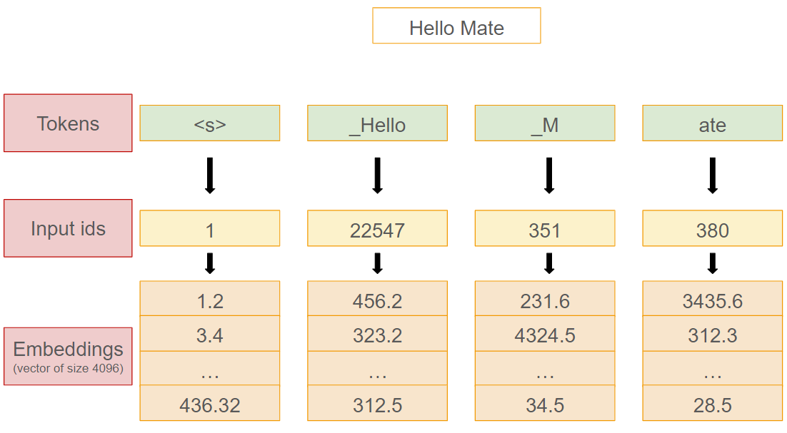
tokenizer("Hello Mate")
{'input_ids': [1, 22557, 351, 380], 'attention_mask': [1, 1, 1, 1]}
tokenizer.convert_ids_to_tokens(tokenizer("Hello Mate")["input_ids"])
['<s>', '▁Hello', '▁M', 'ate']
The tokenizer converts text into a format understandable by the model. The process involves two key elements:
Input Ids#
The tokenizer uses a predefined vocabulary that maps words or subwords to unique integers. In Mistral’s case, the tokenizer encodes “Hello Mate” to [1, 22557, 351, 380]. Each number corresponds to a specific token in the model’s vocabulary (The corresponding vocabulary is (‘<s>’, ‘▁Hello’, ‘▁M’, ‘ate’), where the underscore indicates that there is a whitespace separating the current token from the previous one).
The total vocabulary size is 32k.
Attention Mask#
Along with the input_ids, the tokenizer also generates an attention_mask [1, 1, 1, 1] in this case. The attention mask helps the model understand which tokens should be focused on and which should be ignored (e.g., padding tokens). In this example, all tokens are relevant, so the attention mask is all ones. We will explain in more details how this mask is used when we explain the Attention component in Mistral (here).
Model output#
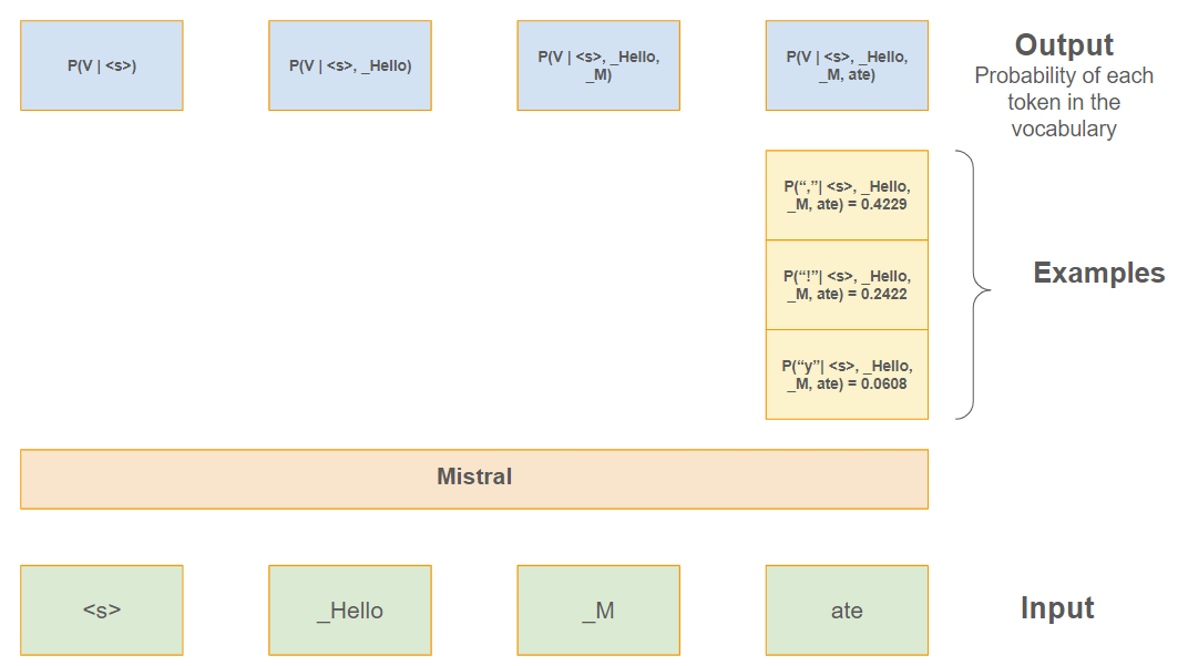
Mistral is an Autoregressive Language Model.
It is pretrained to estimate given a sequence of tokens \(\{y_N,...,y_1\}\):
Take, for instance, the specific sequence \(\{ y_1=\text{"<s>"}, y_2 = \text{"_Hello"}, y_3 = \text{"_M"}, y_4 = \text{"ate"} \}\). The task here is to predict the next token in the sequence, referred to as \(y_5\).
The model evaluates the probability of \(y_5\) being any token from its vocabulary given the preceding sequence. This probability can be written as: \(P(y_5 \in V | y_1=\text{"<s>"}, y_2 = \text{"_Hello"}, y_3 = \text{"_M"}, y_4 = \text{"ate"})\).
An illustrative example is provided below, showcasing the top three most likely candidates for the next token.
If we choose the 3rd most likely next token, we get: “Hello Matey” 🤓.
Input / Output Illustration
We will see (when delving into the architecture details) that the autoregressive property of Mistral is encoded thanks to a trick called Causal Mask.
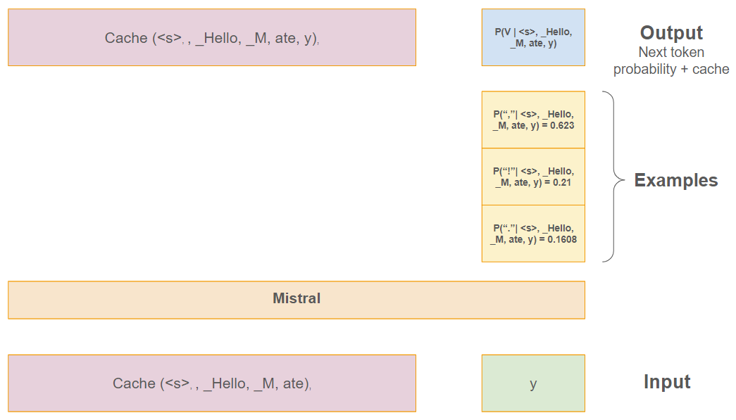
Natural Language Generation, Prompt and Caching#
Mistral, like any autoregressive model generates text by predicting the next token token in a sequence.
It would be inefficient to recalculate for every new tokens the previous calculated distributions.
To avoid recomputing the entire sequence’s representation at each step. Instead, Mistral reuses calculations from previous steps, making the process faster and more resource-efficient.
This component is called the Key-Value cache. We will explain later in details how it works.
For clarity, we excluded the key-value cache component from the prior section’s diagram.
In the same example, if “y” is chosen as the next token in the first prediction phase, it creates the phrase “Hello Matey.”
In the second step, with the cache in use, the model can be depicted as follows:
Input / Output Illustration with Cache
2. Dissecting each layer of Mistral Architecture#
Overall architecture:
Mistral Architecture
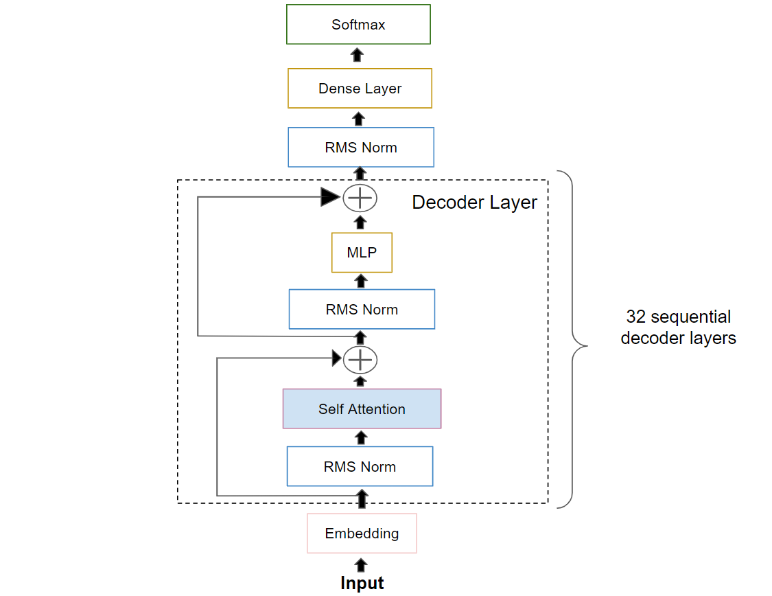
The architecture diagram presents a high-level view of how the Mistral model processes input to generate language.
Key components include:
Input: The starting point for the model where tokenized text is received.
Embedding Layer: Transforms tokens into meaningful vector representations.
Decoder Layers: A critical component of the Mistral model, 32 layers that include:
Self-Attention: A mechanism enabling each position to consider the entire input sequence for context.
RMS Norm: Applied to normalize layer activations, stabilizing the learning process.
MLP (Multi-Layer Perceptron): Processes the attention output using a gated feed-forward neural network.
Add: Incorporates residual connections to assist in training deep networks.
Dense Layer: Shapes the processed data into the final output format.
Softmax: Converts logits into distributions over the vocabulary conditionally on the previous tokens.
To summarize in one formula the model, given n tokens as an input:
Everything up to the last Decoder is what is called MistralModel in 🤗 Hugging Face implementation. The Dense Layer is the Causal Language Modelling head that can be dropped/replaced if we wish to do other tasks than Natural Language Generation ones.
The Self-Attention within the Decoder Layer is particularly crucial, as it directly influences the model’s ability to generate contextually relevant text. It’s this feature that we will explore in greater detail.
Embedding Layer#
In the Mistral model with an embedding dimension (hidden_size) of 4096, the embedding layer transforms an input sequence of length seq_len into a matrix \(E \in M_{\text{seq_len} \times \text{hidden_size}}(\mathbb{R})\).
This matrix represents the embedded representation of each token in the input sequence, where each row of the matrix corresponds to the embedded vector of a token in the sequence.
The illustration below is a visualization for an input sequence where seq_len equals 4.
illustration
Decoder Layer#
For a given sequence length, the decoder layer is an endomorphism \(f : M_{\text{seq_len} \times \text{hidden_size}}(\mathbb{R}) \mapsto M_{\text{seq_len} \times \text{hidden_size}}(\mathbb{R})\).
In other word, it is a function where the input and output spaces have the same dimensions.
This design ensures that the output from one decoder layer can seamlessly serve as the input for the subsequent decoder layer.
Let’s now delve into the most important component: Self-Attention.
Self-Attention#
computation graph
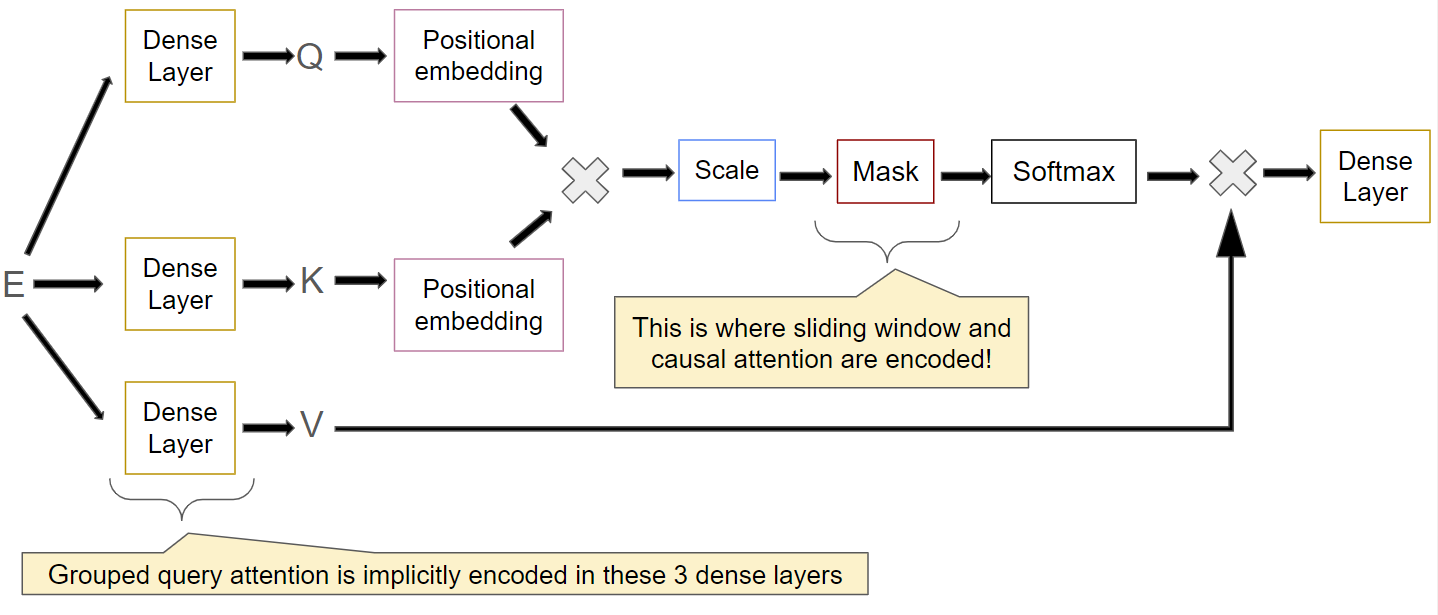
The MistralAttention class in huggingface/transformers is an implementation of a grouped query attention mechanism, integrating concepts from [Vaswani et al., 2017] and sliding window attention techniques from [Beltagy et al., 2020] and [Child et al., 2019].
Parameters#
The attention module is initialized with the following key parameters:
hidden_size: \(d_{\text{model}} = 4096\), the dimensionality of the input feature space (already defined in the embedding layer).num_heads: \(h = 32\), the number of attention heads.head_dim: \(d_k = \frac{d_{\text{model}}}{h} = 128\) the dimensionality of each attention head.num_key_value_heads: \(h_{kv} = 8\), the number of heads used for key and value projections.num_key_value_groups: \(g_{kv} = \frac{h}{h_{kv}} = 4\), the number of groups for key-value heads.max_position_embeddings(32768) andrope_theta(10000): Parameters for rotary position embeddings.
Attention Calculation#
Projection:
The input matrix \(E \in \mathbb{R}^{\text{seq_length} \times d_{\text{model}}}\) (normalized embedding in the first decoder) is linearly projected to query (Q), key (K), and value (V) matrices:
\[\begin{split}Q = E \times W^Q \quad &\text{with} \quad W^Q \in \mathbb{R}^{ d_{\text{model}} \times d_k h} \\ K = E \times W^K \quad &\text{with} \quad W^K \in \mathbb{R}^{ d_{\text{model}} \times d_k h_{kv}} \\ V = E \times W^V \quad &\text{with} \quad W^V \in \mathbb{R}^{d_{\text{model}} \times d_k h_{kv}}\end{split}\]These projections are reshaped and transposed to prepare for the grouped query attention calculation and we obtain the following matrices:
\(Q = (Q_1 | ... | Q_{h=32}) \text{ where } Q_i \in \mathbb{R}^{\text{seq_length} \times d_k}\)
\(K = (K_1 | ... | K_{h_{kv}=8}) \text{ where } K_i \in \mathbb{R}^{\text{seq_length} \times d_k}\)
\(V = (V_1 | ... | V_{h_{kv}=8}) \text{ where } V_i \in \mathbb{R}^{\text{seq_length} \times d_k}\)
Rotary Position Embedding:
Rotary embeddings are applied to Q and K to incorporate positional information.
Let \(q_{j}\) be the \(\text{j}^{th}\) row of \(Q_i\). In the first decoder, this encodes information of the \(\text{j}^{th}\) token.
Let \(k_{l}\) be the \(\text{l}^{th}\) row of \(V_i\).In the first decoder, this encodes information of the \(\text{l}^{th}\) token.
The idea of the Rotary position embedding [Su et al., 2023] is to transform \(\tilde{q}_{j} = f(q_{j}, j)\) and \(\tilde{k}_{l} = f(k_{l}, l)\) such that the inner product only depends on the relative position between k and l:
\[\tilde{q}^{t}_{j} \tilde{k}_{l} = g( q_{j}, k_{l}, j-l)\]You may wonder why we are using the inner-product. To answer this, we need to look ahead. The mth row of the calculated Attention Score (detailed in item 4 below) is:
\[\text{Attention}_{m}(Q, K, V) = \sum_{i=1}^{m}\frac{\exp(\frac{q_{m}^{t}k_{i}}{\sqrt{d_k}}) }{\sum_{j=1}^{m}\exp(\frac{q_{m}^{t}k_{j}}{\sqrt{d_k}})}v_{i}\]Combining the formulas above, we get a self-attention mechanism that takes into account the relative position between tokens j and l:
\[\text{Attention}_{m}(\tilde{Q}, \tilde{K}, V) = \sum_{i=1}^{m}\frac{\exp(\frac{\tilde{q}^{t}_{m}\tilde{k}_{i}}{\sqrt{d_k}}) }{\sum_{j=1}^{m}\exp(\frac{\tilde{q}^{t}_{m}\tilde{k}_{j}}{\sqrt{d_k}})}v_{i}\]In addition the function that is chosen in [Su et al., 2023] has the property of a long-term decay property, which means the inner-product will decay when the relative position increases.
For more details about the exact formula applied in ROPE, please refer to the paper [Su et al., 2023] or this great post.
Grouped query attention preparation
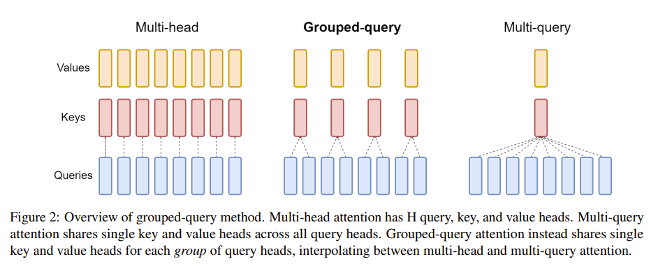
Source: [Ainslie et al., 2023]#
The key and value tensors are repeated to prepare for the grouped self-attention computation:
\(\tilde{K} = (\tilde{K}_1 | \tilde{K}_1 | \tilde{K}_1 | \tilde{K}_1 | ... | \tilde{K}_{8}| \tilde{K}_{8} | \tilde{K}_{8}| \tilde{K}_{8}) \text{ where } K_i \in \mathbb{R}^{\text{seq_length} \times d_k}\)
\(V = (V_1 | V_1 | V_1 | V_1 | ... | V_{8}| V_{8} | V_{8}| V_{8}) \text{ where } K_i \in \mathbb{R}^{\text{seq_length} \times d_k}\)
Attention Score Calculation:
Attention scores are calculated using the scaled dot-product attention mechanism, for a given triple \((Q_i, K_i, V_i)\):
(1)#\[\text{Attention}(\tilde{Q}_i, \tilde{K}_i, V_i) = \text{softmax}\left(\frac{\tilde{Q}_i\tilde{K}_i^T}{\sqrt{d_k}} + \text{Mask}\right)V_i\]The softmax is applied across the last dimension of the scaled dot-product.
You may have noticed that we have introduced a new matrix called Mask in the softmax. This is where the causal attention mechanism and the sliding window attention are implemented.
This is done by setting the value of an element of \(\tilde{Q}\tilde{K}^T\) to \(-\infty\) before the softmax so that attention weights become 0 since \(\exp(-\infty)=0\) and softmax is a normalized exponential.
For mistral, we can decompose the mask into the sum of three matrices \(\text{Mask} = \text{Mask}_{\text{Causal}} + \text{Mask}_{\text{Sliding Window}} + \text{Mask}_{\text{Attention}}\):
Causal Mask: Remember that Mistral is an autoregressive meaning that it is pretrained to estimate given a sequence of tokens \(\{y_N,...,y_1\}\): \(P(y_N,...,y_1) = \prod_{n-1}^{N} P(y_t | y_{<t})\). The causal mask is here to encode this autoregressive property:
\[\begin{split}\begin{bmatrix} 0 & -\infty & -\infty & \cdots & -\infty \\ 0 & 0 & -\infty & \cdots & -\infty \\ 0 & 0 & 0 & \cdots & -\infty \\ \vdots & \vdots & \vdots & \ddots & \vdots \\ 0 & 0 & 0 & \cdots & 0 \\ \end{bmatrix} \in \mathbb{R}^{\text{seq_length} \times \text{seq_length}}\end{split}\]Sliding window Mask: A matrix of 0s if seq_length is inferior to the window size 4096, else:
\[\begin{split}\begin{bmatrix} 0 & \overbrace{ \cdots }^{\text{ window size} -2} & 0 & -\infty & -\infty & \cdots & -\infty \\ -\infty & 0 & \cdots & 0 & 0 & -\infty & \cdots & -\infty \\ -\infty & -\infty & \ddots & \vdots & \vdots & \ddots & \ddots & \vdots \\ -\infty & -\infty & \cdots & 0 & 0 & 0 & \cdots & -\infty \\ -\infty & -\infty & \cdots & -\infty & 0 & 0 & \cdots & 0 \\ \vdots & \vdots & \ddots & \vdots & \vdots & \vdots & \ddots & \vdots \\ -\infty & -\infty & \cdots & -\infty & -\infty & -\infty & \cdots & 0 \\ \end{bmatrix}\end{split}\]Attention mask: Let’s say that my attention mask is [0, 0, 1, 1, 1], where 0 means don’t attend. The mask associated to it would be:
\[\begin{split}\begin{pmatrix} -\infty & -\infty & -\infty & -\infty & -\infty \\ -\infty & -\infty & -\infty & -\infty & -\infty \\ -\infty & -\infty & 0 & 0 & 0 \\ -\infty & -\infty & 0 & 0 & 0 \\ -\infty & -\infty & 0 & 0 & 0 \\ \end{pmatrix}\end{split}\]Output Projection:
Finally, the attended output is projected back to the original dimension
hidden_size:\[\text{Output} = \text{Attention}(\tilde{Q}, \tilde{K}, V) \times W^O \quad \text{with} \quad W^O \in \mathbb{R}^{d_k h \times d_{\text{model}}}\]
If attention is all you need why do we have RMSNorm, Residual Connection and a MLP?#
RMSNorm: Data normalization to stabilize learning#
RMSNorm is designed to normalize the activations of a layer within a neural network to stabilize the learning process.
Please refer to [Zhang and Sennrich, 2019] for more details.
Residual Connections: helping to train deep networks#
The original “Attention is All You Need” [Vaswani et al., 2017] paper already incorporated residual connections and MLPs, though Mistral uses a distinct activation function in the gated feed-forward network.
Residual connections were introduced in [He et al., 2016] with the intuition that learning \(F_l(x_{l-1}) = x_{l} -x_{l-1}\) instead of \(F_l(x_{l-1}) = x_{l}\) makes it easy to learn the identity function and hence helps achieving at least the same performance as the same network with less layers.
[Li et al., 2018] developed a way to visualize error surfaces and shown that residual connections help to smooth the error surface.
MLP: adding non-linearity#
Attention mechanism creates linear combinations of the value vectors and values are linear functions of the inputs. As a result, the output of an attention layer is constrained to be a liner combination of the input.
Hence a non-linear function like a Multi-Layer Perceptron (MLP) helps to add non-linearity to the model.
[Dong et al., 2021] shown that in the absence of skip connections or MLPs, the output tends to rapidly converge to a rank 1 matrix. The presence of skip connections and MLPs helps prevent this degradation of the output.
For further details on architecture choices related to transformers, you can refer to [Lin et al., 2022].
3. Important Implementation Details#
Key-Value Cache#
Motivation: NLG task Inference#
Natural Language Generation tasks inherently involve generating tokens one at a time, in a sequential manner. To optimize this process, it’s crucial to minimize redundant computations. Specifically, our goal is to avoid recalculating the entire sequence of hidden states each time we add a new token.
We have seen so far in the previous section that the model input-output is:
However in a sequential scenario (one token at a time) we only need \(P(y_{n+1} | y_{<n+1})\) since the other probabilities have already been computed.
The cache consist in implementing a function that only processes the latest token while utilizing previously stored computational elements:
This optimization more precisely happens in the self-attention layer. We have omitted it in the previous section for clarity. Let’s see now how it works.
Attention Key-Value Cache#
As a reminder, Attention is calculated as follow:
Consider a scenario with n+1 tokens. The query key matrix multiplication can be represented as follow:
In the matrix above, notice that:
The blue elements represent computations already performed in the previous step with n tokens.
The green elements are equal to minus infinity due to the causal mask.
As a result, the only part that needs to be calculated is represented in red and does not need \(\{q_1,...q_n\}\).
The full attention calculation with a causal mask can be expressed as follow:
You might have noticed that elements in blue sum to up to n, this is thanks to the causal mask.
As a result, attention for to tokens 1 to n is already calculated in previous steps.
Therefore, at step n+1, we only need to calculate the red element \({\color{red}\sum_{i=1}^{n+1}\frac{\exp(\frac{q_{n+1}k_{i}}{\sqrt{d_k}}) }{\sum_{j=1}^{n+1}\exp(\frac{q_{n+1}k_{j}}{\sqrt{d_k}})}v_{i}}\).
To achieve this, we only need to stores the Key and Value matrices and performs the matrix multiplication with \(q_{n+1}\) for the new calculations.
We do not need to cache previous attentions since our aim is to compute the probability of the next token and since we have already calculated them in the previous step.
In summary, at step n + 1, we take \(k_{n+1}\) and \(v_{n+1}\) and append these to the cached keys and values (\(K_{1:n}\)) and values (\(V_{1:n}\)):
With caching, attention is computed as:
Cache and Sliding window: Rolling Buffer Cache
The sliding window allows us to be even more memory efficient by storing only up to the last window_size elements of the Key and Value Matrices.
On a sequence length of 32k tokens and a window size of 4096, this reduces the cache memory usage by 8x, without impacting the model quality.
Padding#
Important notes on the tokenizer effect on model output#
To pad or not to pad (be careful if you use a 🤗 Hugging Face trainer when fine tuning a Language Model)
In the Mistral tokenizer, there’s no specific padding token. Padding tokens are crucial for encoding batches with sequences of varying lengths, as they standardize input size by filling in shorter sequences to match the longest one in the batch.
A common workaround that I see in many codebases and tutorials that fine-tune a model with a 🤗 Hugging Face trainer is setting tokenizer.pad_token = tokenizer.eos_token. However, be aware of its effect if you are planning to fine-tune your model. The End-of-Sequence (EoS) token plays a vital role in signaling the model to stop generating further tokens. When the padding token is set to the same value as the EoS token, the model’s ability to learn when to appropriately end its output is compromised if the same label is assigned during training time. This issue can lead to unintended model behavior during inference. For example, if the model cannot recognize the end of a sequence, it might continue generating tokens indefinitely. This might result in the model producing lengthy, nonsensical outputs or simulated conversations, which are far from the desired single instruction response.
To understand why:
The pad_token_id in hugging face is being assigned the label ignore_index in the loss function below:
\[\begin{split}\ell(x, y) = - \sum_{n=1}^N \mathbb{1}_{y_n \not= \text{ignore_index}} \log \frac{exp(x_{n,y_n})}{\sum_{c=1}^{C} exp(x_{n,c})} \\\end{split}\]where:
x = (x_1, …, x_N) represents the logits output of a Mistral model for an input of sequence N + 1
y = (y_1, …, y_N) their respective labels
Therefore if you set tokenizer.pad_token to tokenizer.eos_token, we are assigning eos_token_id to pad_token_id, as a result all eos tokens will be ignored in the loss function.
What should you do then?
Avoid Padding When Possible: One way to achieve this is by using a ConstantLengthDataset or similar approaches where all input sequences are pre-processed to have a uniform length. This method eliminates the need for dynamic padding during training.
Add a Padding Token if Necessary: In cases where you cannot avoid variable-length sequences and padding becomes essential, you can add a padding token to your tokenizer. This can be done using the add_special_tokens method: tokenizer.add_special_tokens({‘pad_token’: ‘[PAD]’}). This method adds a new special token [PAD] to the tokenizer, which you can then use as a padding token. You will have however to resize your embedding layer to factor adding a new token in the vocabulary.
Handle labels correctly and prefer other frameworks than hugging face trainers (by using pytorch code directly or pytorch lightning).
How to cite this post?#
@article{filali2023mistral,
  title   = "Mistral: Decoding the Complexities of a Large Autoregressive Language Model",
  author  = "FILALI BABA, Hamza",
  journal = "hamzaonai.com",
  year    = "2023",
  month   = "Dec",
  url     = "https://hamzaonai.com/blog/llm_mistral.html"
}
References#
- ALTdJ+23
Joshua Ainslie, James Lee-Thorp, Michiel de Jong, Yury Zemlyanskiy, Federico Lebrón, and Sumit Sanghai. Gqa: training generalized multi-query transformer models from multi-head checkpoints. arXiv preprint arXiv:2305.13245, 2023.
- BPC20
Iz Beltagy, Matthew E Peters, and Arman Cohan. Longformer: the long-document transformer. arXiv preprint arXiv:2004.05150, 2020.
- CGRS19
Rewon Child, Scott Gray, Alec Radford, and Ilya Sutskever. Generating long sequences with sparse transformers. arXiv preprint arXiv:1904.10509, 2019.
- DCL21
Yihe Dong, Jean-Baptiste Cordonnier, and Andreas Loukas. Attention is not all you need: pure attention loses rank doubly exponentially with depth. In International Conference on Machine Learning, 2793–2803. PMLR, 2021.
- HZRS16
Kaiming He, Xiangyu Zhang, Shaoqing Ren, and Jian Sun. Deep residual learning for image recognition. In Proceedings of the IEEE conference on computer vision and pattern recognition, 770–778. 2016.
- JSM+23
Albert Q Jiang, Alexandre Sablayrolles, Arthur Mensch, Chris Bamford, Devendra Singh Chaplot, Diego de las Casas, Florian Bressand, Gianna Lengyel, Guillaume Lample, Lucile Saulnier, and others. Mistral 7b. arXiv preprint arXiv:2310.06825, 2023.
- LXT+18
Hao Li, Zheng Xu, Gavin Taylor, Christoph Studer, and Tom Goldstein. Visualizing the loss landscape of neural nets. Advances in neural information processing systems, 2018.
- LWLQ22
Tianyang Lin, Yuxin Wang, Xiangyang Liu, and Xipeng Qiu. A survey of transformers. AI Open, 2022.
- SAL+23(1,2,3)
Jianlin Su, Murtadha Ahmed, Yu Lu, Shengfeng Pan, Wen Bo, and Yunfeng Liu. Roformer: enhanced transformer with rotary position embedding. Neurocomputing, pages 127063, 2023.
- VSP+17(1,2)
Ashish Vaswani, Noam Shazeer, Niki Parmar, Jakob Uszkoreit, Llion Jones, Aidan N Gomez, Łukasz Kaiser, and Illia Polosukhin. Attention is all you need. Advances in neural information processing systems, 2017.
- ZS19
Biao Zhang and Rico Sennrich. Root mean square layer normalization. Advances in Neural Information Processing Systems, 2019.