Dropout as a way to Model Uncertainty in Deep Learning Models#
Introduction#
In [Gal and Ghahramani, 2016], the authors propose an easy, fast and scalable method to quantify the uncertainty of any deep learning model (including big modern architectures) as long as dropout is used during training time.
We are going to summarize in this post how the authors arrive to this conclusion while highlighting the main approximations made to reach this conclusion.
The key concept is that during training time of a deep learning model with dropout, minimizing the loss function is approximately equivalent to obtaining a variational approximation of a deep gaussian process (using approximately the dropout distribution as a variational law).
We have used twice the word approximation. Let’s look at the approximations involved with a simple example: a single hidden layer neural network.
Notations#
- Let \(y = σ(xW1 + b)W2\) be the output of our single hidden layer NN, given:
some input \(x \in \mathbb{R}^{Q}\)
the bias term \(b \in \mathbb{R}^{K}\)
the weight matrices connecting the first layer to the hidden layer \(W_{1} \in \mathbb{R}^{Q \times K}\)
the weight matrices connecting the hidden layer to the output layer \(W_{2} \in \mathbb{R}^{K \times D}\)
Let \(X = \{x_1, ... , x_N \}\), \(Y = \{y_1, ... , y_N \}\) be our training set.
Let \(\omega = \{W_{1}, W_{2}, b\}\) denote the weight parameters of our Neural Network.
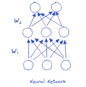
Dropout illustration#
Modelling uncertainty through the concept of Bayesian predictive probability#
Given a new input \(x^*\), we would like to estimate the predictive probability:
Below is a summary of the approximations that we will explain in the following sections:
Gaussian Process Approximation#
In a Gaussian Process we need to define the a covariance function. Which can be defined in our neural network as \(K(x, y) = \int \mathcal{N}(w; 0,l^{-2}I_Q) p(b) \sigma(w^T x + b) \sigma(w^T y + b) d w d b\).
By approximating this covariance function with: \(\hat{K}(x, y) = \frac{1}{K} \sum_{k=1}^K \sigma(w_k^T x + b_k) \sigma(w_k^T y + b_k)\) where \(w_k \sim \mathcal{N}(0,l^{-2}I_Q)\) and \(b_k \sim p(b)\).
The authors show in section 3.1 of the appendix [Gal and Ghahramani, 2016] that this approximation leads to:
Variational inference recipe#
A variational distribution \(q_\theta(\omega)=q_\theta(W_1)q_\theta(W_2)q_\theta(b)\) is used to approximate the posterior \(p(\omega | X, Y)\):
For \(W_1\), we set:
\(\quad\) \(\quad\) where \(p_1 \in [0, 1]\), \(\sigma > 0\) and \(M_1 = [m_q]_{q=1}^Q \in \mathbb{R}^{Q \times D}\) variational parameters.
We repeat the same for \(W_2\). Our set of variational parameters is then defined as \(\theta = \{ M_1, M_2, m, p_1, p_2, \sigma \}\), with \(M_2\) the variational parameter for \(W_2\) and \(m\) the variational parameter for \(b\).
We set \(\sigma\) very close to zero (e.g. 10 power -33 to be lower than a machine precision). This means that sampling programmatically from the gaussian mixture leads to sampling from a Bernoulli random variable that returns either 0 with probability \(1−p_1\) or \(m_k\) with probability \(p_1\), which is equivalent to applying dropout to the weights of the model.
Minimizing the kullback leibler divergence is equivalent to minimizing minus the log evidence lower bound with respect to \(\theta\), i.e.: \(argmin_\theta KL(q_\theta(\omega) || p(\omega | X, Y)) = argmin_\theta \mathcal{L}_{\text{VI}}\). The authors use a one sample monte carlo approximation of the log evidence lower bound and show that it is proportional to the loss function of the neural network with parameters \(\theta\):
Point 5 proves that minimizing the loss function of a single hidden layer NN with dropout activated at training time, leads also to a variational approximation of our bayesian model, where the variational distribution is the same dropout distribution.
Conclusion#
We have highlighted the approximations that lead to the bayesian conclusion at inference time that : \(p(y^* | x^*, X, Y) \approx \int p(y^* | x^*, \omega) q_{\theta}(\omega)d \omega\) where \(\theta\) are the weights of the model and the dropout parameters obtained at training time \(\{ M_1, M_2, m, p_1, p_2\}\).
An easy, fast and scalable method to quantify the uncertainty is to finally use a finite sample estimate of our model uncertainty with K dropout passes which leads to \(p(y^* | x^*, X, Y) \approx \frac{\sum_{i=1}^{T} p(y^* | x^*, \omega_t)}{T}\).
References#
- Gal16
Yarin Gal. Uncertainty in Deep Learning. PhD thesis, University of Cambridge, 2016.
- GG16(1,2)
Yarin Gal and Zoubin Ghahramani. Dropout as a bayesian approximation: representing model uncertainty in deep learning. In international conference on machine learning, 1050–1059. PMLR, 2016.
- GIG17
Yarin Gal, Riashat Islam, and Zoubin Ghahramani. Deep bayesian active learning with image data. In International conference on machine learning, 1183–1192. PMLR, 2017.
- Gal86
Francis Galton. Regression towards mediocrity in hereditary stature. The Journal of the Anthropological Institute of Great Britain and Ireland, 15:246–263, 1886.