Notes on Bayesian Online Change Point Detection#
In this post we are going to delve into the mathematical details behind the graphical model Bayesian Online Change Point Detection introduced in [Adams and MacKay, 2007]. This model can be used to detect different type of change-points and has known many extensions over the last few years.
Given a time series, we are interested in detecting structural changes as new data comes in.
A great explanation of this paper can be found in [Gundersen, 2022].
You might ask, why reading this post then? There is three main reasons.First, I will try to clarify parts that were not trivial to me despite reading the paper and the post above (e.g. a tiny mistake was made in the math derivation).
Second and most importantly the paper only provides a way to calculate the probability that there was a change-point k units of time ago, but it does not propose a strategy to segment the time-series. I will suggest an algorithm to perform an optimal segmentation at a given time t. Finally, I will show how we can use BOCPD to detect trend changes.
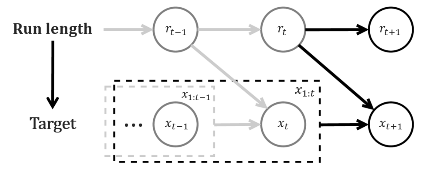
Graphical model associated to BOCPD. Source [Kim and Choi, 2015]#
BOCPD#
Let \(\{x_{1}, ... x_{T}\} \in \mathbf{R}^{T\times d}\) denote the time series of interest.
Introducing the main ingredient: Run-length#
Let \(r_{t}\), the run-length, be a random variable that represent the time since the last change-point. For instance, \(r_{t} = j\) implies that the last change-point was at time \(t-j\).
It follows that \(r_{t} \in \mathbf{R}^{t}\) and \(r_{t} = \begin{cases} 0 \text{ if change-point at time t} \\ r_{t-1} + 1 \text{ else} \end{cases}\).
In the BOCPD model, our main interest lies in calculating the run-length posterior distribution \(P(r_{t}|x_{1:t})\).
In order to compute it we need to make some assumptions around:
the conditional dependence structure between \(\{x_{1}, ... x_{T}\}\) and \(\{r_{1}, ... r_{T}\}\)
the underlying distribution of \(\{x_{1}, ... x_{T}\}\) and \(\{r_{1}, ... r_{T}\}\)
Conditional dependence structure assumptions#
The assumptions that we are going to explain in more details are outlined in the graphical representation above.
Assumption 1:
We assume that \(r_{t}\) is conditionally independent of everything else given \(r_{t-1}\). In particular, \(P(r_{t} | r_{t-1}, x_{1:t}) = P(r_{t} | r_{t-1})\)
Assumption 2:
We assume that the current observation only depends on the past observations associated to the current partition defined be the run-length, i.e. \(P(x_{t} | r_{t-1}=r, x_{1:t-1}) = P(x_{t} | x_{t-r-1:t-1})\)
With these two assumptions, we can derive our main objective \(P(r_{t}|x_{1:t})\).
Given that \(P(r_{t}|x_{1:t}) = \frac{P(r_{t},x_{1:t})}{\sum_{r'_{t}}P(r'_{t},x_{1:t})} \tag{1}\).
Three terms appear in the equations above:
We now need to make assumptions on the distribution of the Change-point Prior and the Underlying Predictive Model in order to be able to recursively derive the run-length posterior.
Underlying distribution assumptions#
Change-point prior model#
The transition probability \(P(r_{t}|r_{t-1})\) is assumed to follow the below distribution:
where \(H(\tau) = \frac{p_{g}(\tau)}{\sum_{t=\tau}^{\infty}p_{g}(t)}\) is the hazard function[^2] and \(p_{g}(t)\) represents the probability of a segment of length t.
If we set \(p_{g}\) to follow a geometric distribution with parameter \(\lambda\) then \(H(\tau) = \frac{1}{\lambda}\). The prior \(\lambda\) encodes our belief on the expected length of a segment, in other words our prior on the average length of a partition.
Predictive Model assumptions#
The last part we need to compute is the predictive probability \(P( x_{t} | r_{t-1}, x_{t-1- r_{t-1}:t-1})\).
Assumption 3:
We assume that \(x_{t}\) follows a distribution with parameter \(\eta\) (where \(\eta\) is a random quantity in a bayesian framework). \(\eta\) is shared across all the \(x_{i}\) within a segment (defined by the run-length).
Given our new point, we are trying to estimate the probability that this new point belongs to the current partition:
Assumption 4:
\(x_{t} \perp\kern-5pt\perp r_{t-1}, x_{t-1- r_{t-1}:t-1} |\eta.\)
Under this assumption, we obtain:
\(P( x_{t} | r_{t-1}, x_{t-1- r_{t-1}:t-1}) = \int \underbrace{P( x_{t}| \eta)}_\text{underlying model} \underbrace{P( \eta | r_{t-1}, x_{t-1- r_{t-1}:t-1})}_{\text{Posterior Distribution}}d \eta\)
We now need to define the underlying distribution of our time series and the distribution of the prior \(\eta\).
The law \(x_{t} | \eta\) that we choose defines the type of change-points we wish to detect.
If we are interested in detecting abrupt shifts in the mean, we could then choose a Gaussian distribution.
If we have count data, we could be tempted to choose a Poisson distribution.
If we have are interested in changes in the trend, we could choose a Bayesian linear regression with time as a regressor.
In [Adams and MacKay, 2007], \(x_{t}| \eta\) is restricted to come from the Exponential Family and the prior \(P(\eta)\) is restricted to be a conjugate prior (which means that \(P( \eta | r_{t-1}, x_{t-1- r_{t-1}:t-1})\) and \(P(\eta)\) come from the same family distribution).
The choice of Exponential family + conjugate prior is motivated by a trade-off between tractability of the equations and generalization over the type of change-points that can be detected:
The conjugate prior allows for a tractable derivation of the posterior distribution as we obtain a closed-form of the posterior distribution. The main derivation needed is on the hyper-parameters associated with the posterior distribution. In the case of an Exponential Family likelihood, the hyper-parameters have an easy formula that can be updated sequentially, a very appealing property in the case of sequential learning.
The Exponential Family encompasses a lot of widely used family for change-point detection problems (e.g. normal distribution, poisson distribution, bayesian linear regression...).
Most of the exponential family distributions lead to a closed form of the predictive probability when the prior is conjugate, which avoids us to resort to bayesian approximation techniques that are computationally costly.
How can we use the output of BOCPD to detect changes?#
An offline strategy: a viterbi-like algorithm#
A natural criteria to find the best segmentation up until time t is to find the Maximum A Posteriori sequence of run-length, i.e. the most probable sequence of run-length:
\(r^{*}_{1}, ... r^{*}_{t} = \arg \max\limits_{r_{1}, ... r_{t}} P(r_{1}, ... r_{t} | x_{1}, ..., x_{t})\)
By noticing that:
We will optimize \(P(r_{1}, ... r_{t} , x_{1}, ..., x_{t})\) through a dynamic programming algorithm.
This optimization formulation is the same as the Viterbi Algorithm used for Hidden Markov Models (see e.g. chapter 17 of [Murphy, 2012]).
However, the structural dependencies are slightly different, hence the recursion is slightly different.
The graphical model above illustrates the structural dependencies assumptions in BOCPD, which are used in the last line of the equation below.
Now let’s introduce a few notations:
Let \(\delta_{t}(j) \overset{\Delta}{=} \log P(r_{1}, ..., r_{t}=j, x_{1}, ..., x_{t})\).
Let \(A(i,j) \overset{\Delta}{=} \log P(r_{t}=j|r_{t-1}=i)\).
Let \(\lambda_{t}(i) \overset{\Delta}{=} \log P( x_{t}| r_{t-1}=i, x_{1}, ..., x_{t-1})\).
Using the equation above, we get:\(\delta_{t}(j) = \max\limits_{i} A(i,j) + \lambda_{t}(i) +\delta_{t-1}(i)\)
This recursion above allows us to compute the optimal sequence of run-length at each time step.
\(\text{Because } r_{t} = \begin{cases} 0 \text{ if change-point at time t} \\ r_{t-1} + 1 \text{ otherwise} \end{cases}\), it follows that:
Computational aspects#
An important drawback is the time and space complexity of this algorithm. The space complexity and time complexity is \(O(T^{2})\).
An online strategy#
In the online change-point setting, we are above all interested in detecting a new change-point with minimum delay (more than finding retrospectively the optimal segmentation).
An easy and natural strategy would be to detect an alert if the run-length posterior distribution \(P(r_{t} = l| x_{1}, ..., x_{t}) > \text{threshold}\).
There is two parameters to consider here. The parameter \(l\) directly encodes the detection delay with which we will flag a change-point. The threshold encodes the confidence degree with which we will flag a change-point.
One issue with this methodology is that we will generally detect multiple consecutive change-points.
References#
- AM07(1,2)
Ryan Prescott Adams and David JC MacKay. Bayesian online changepoint detection. arXiv preprint arXiv:0710.3742, 2007.
- Gun22
Gregory Gundersen. Bayesian online changepoint detection. 2022. URL: https://gregorygundersen.com/blog/2019/08/13/bocd/.
- Mur12
Kevin P Murphy. Machine learning: a probabilistic perspective. MIT press, 2012.
How to cite this post?#
@article{filali2022bocpd,
  title   = "Notes on Bayesian Online Change Point Detection",
  author  = "FILALI BABA, Hamza",
  journal = "hamzaonai.com",
  year    = "2022",
  month   = "Sept",
  url     = "https://hamzaonai.com/blog/bocpd.html"
}